Archive for the 'General' Category
Progressive Photon Mapping
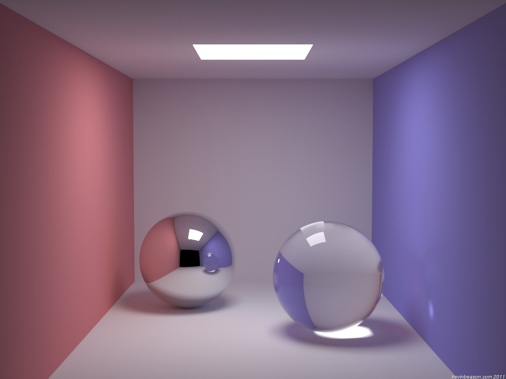
In 2011 I added the progressive version of photon mapping from “Progressive Photon Mapping: A Probabilistic Approach” by Knaus and Zwicker.
The technique is simple and easy to implement but also amazing. Great bang to buck ratio! For anyone starting off with photon mapping, once you have direct visualization of the photon map I would skip irradiance caching and final gathering and just do this. It’s a lot easier, better looking, and still pretty fast.
Here are some test renders. The Cornell Box took about 9 hours for 50,000 passes with 100,000 photons per pass. The Cubo prism took about 18 hours for 50,000 passes using 200,000 photons per pass. Both were done on an Intel i7 920 CPU at 2.67GHz (4 physical cores, 8 logical).
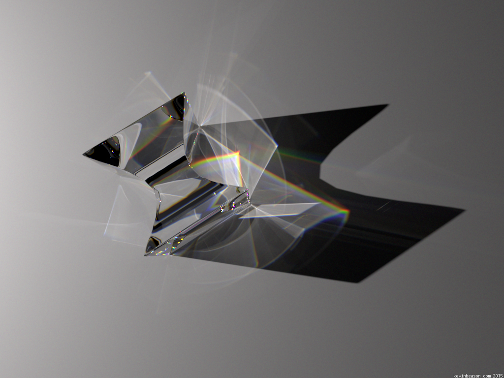
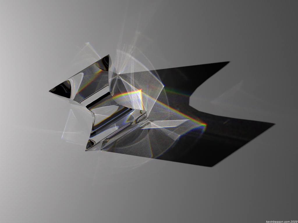
The Cubo prism image looks a lot better than my earlier rendering of it. The caustic is cleaner and the bright reflections of the light are visible.
-

- Cornell Box using PPM
-
- Cubo Prism using PPM
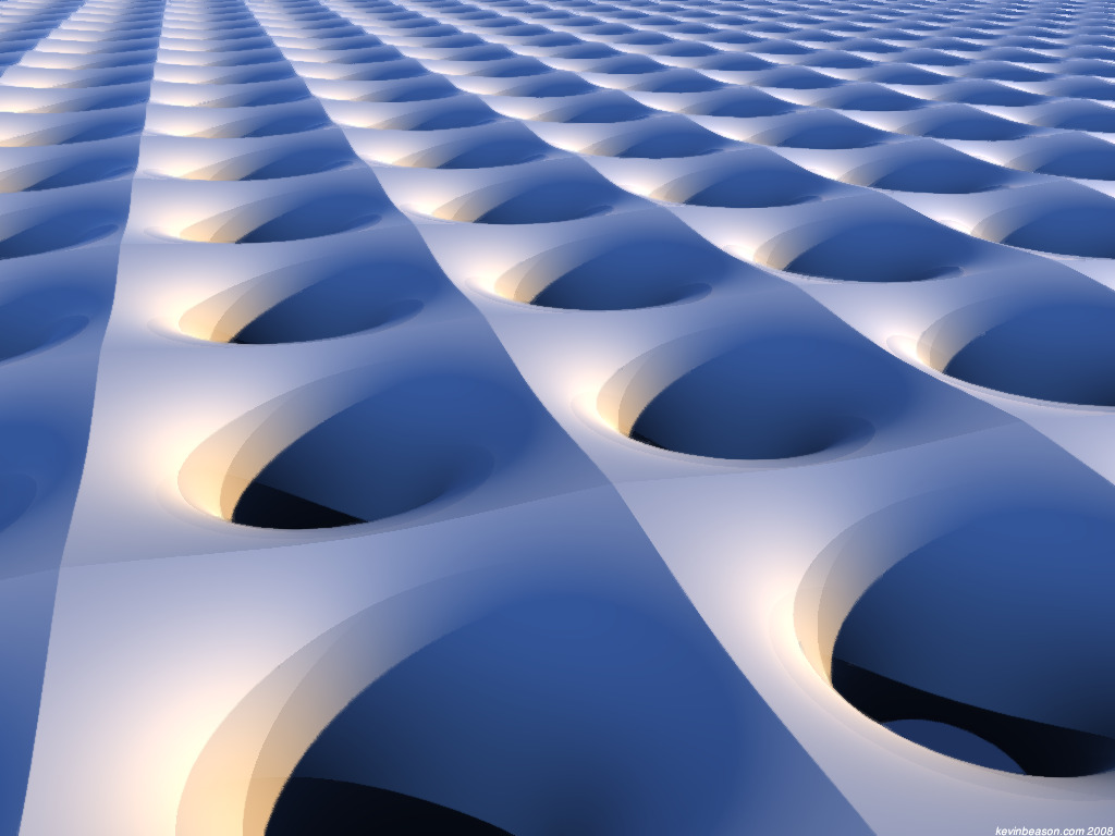
Dispersion, Spectral Filtering, Subpixel Sampling
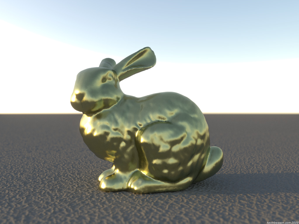
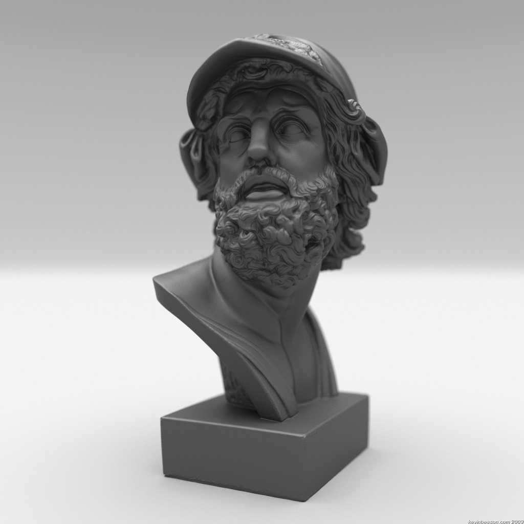
Bunny model available here. Ajax bust available here (thanks jotero!). Bunny scene was under 3 hours, Ajax scene was 8 hours.
The Cubo prism model is available here. For comparison, here is a proper rendering by luxrender. The prism shows off a new feature, spectral rendering. I used 20,000,000 photons which took about 1h20m to emit, and another 10 hours for rendering. (Without diffuse final gather it renders in about 2.5 hours.)
Dispersion in the glass is computed using Cauchy’s equation with dense flint glass (SF10) coefficients. Spectral computations are done in a way similar to this project, but with support for arbitrary wavelengths. I sample a wavelength from the visible spectrum and compute a “wavelength filter”, which is just an RGB color. I convert the CIE XYZ response for that wavelength to RGB and normalize such that a uniform sampling of the entire spectrum produces white (1, 1, 1) instead of (0.387463, 0.258293, 0.240652). Then I scale the emitted photon color and primary rays’ radiance by the normalized color. I sample the wavelengths with importance sampling according to the average CIE XYZ response.
With this spectral filtering I have to take more samples to eliminate the chromatic noise, but the result is consistent with the non-spectral result, provided there is no wavelength dependent reflection such as dispersion. That is, without dispersion, the spectral and non-spectral results match. If there is wavelength dependent reflection, then you get results like the prism image.
Finally, the cubo prism image and the last batch of sphere BRDF tests use subpixel sampling (similar to what’s done in smallpt). I divide each pixel up into 4×4 subpixels. Basically I scale the image resolution by 4, render, do all the tone mapping, and then shrink the image back down to the desired resolution using averaging. This produces much sharper results at the cost of increased memory usage. This is partially based on what Sunflow does, whose source I used as a guide, but without the adaptive anti-aliasing.
9 commentsMultiple Importance Sampling

Fixed lots of bugs in my Ashikhmin & Shirley and Schlick BRDF’s. Schlick anisotropic is still not 100% correct. Added explicit BRDF calculation for both BRDF’s, allowing for light sampling in addition to BRDF importance sampling. This helped a great deal with small light sources like the sun. To incorporate the benefits of both sampling strategies (light and BRDF), I also added Multiple Importance Sampling (MIS) using the one-sample model and balance heuristic as described in section 9.2.4 of Eric Veach’s dissertation. This solves the glossy highlights problem (section 9.3.1).
The MIS is actually incredibly simple to do, once you can compute the BRDF for an arbitrary direction. Choose weights for two sampling strategies (light sampling or brdf sampling). I do .5 and .5. Then select one of the sampling techniques according to its weight. Trace the ray and compute the BRDF. Then divide by the PDF as done for regular importance sampling, but now the PDF is weight1*pdf1+weight2*pdf2 (regardless of technique chosen). Done. Well… actually, it took some refactoring and debugging in lots of places to add MIS everywhere.
I was hung up for a long time because I tried to be cheap and only compute the simplified BRDF/PDF ratio when importance sampling the BRDF. Pointless. Just compute both the BRDF and PDF, since you’ll need both for MIS.
Also added direct lighting computation for emissive spheres.
Times are about 42 minutes with 1024 samples per pixel (spp), on a Q6600 quad core cpu.
5 commentsDistance Field Experiments
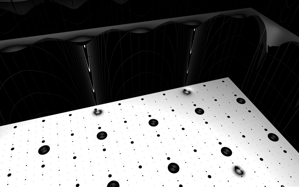
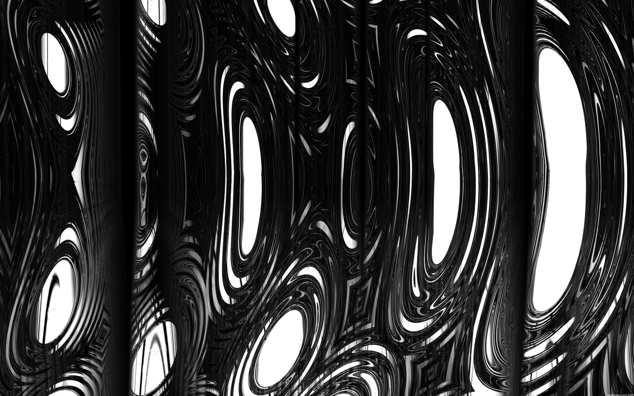
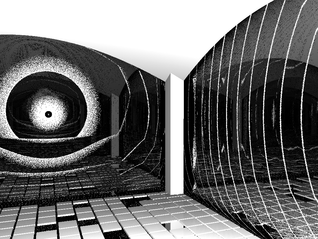
Here are the results from some distance field intersection experiments.
Inspired by slisesix by Inigo Quilez. A better explanation is on my reading list.
I also posted these on ompf. A single sample at 1024×768 takes about 6 seconds on a 2.4GHz Q6600 quad core CPU. Intersection works by stepping the field distance with a minimum step until the isosurface is intersected, and then the distance is refined with bisection method.
Glossy reflections
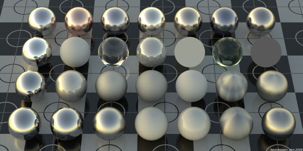
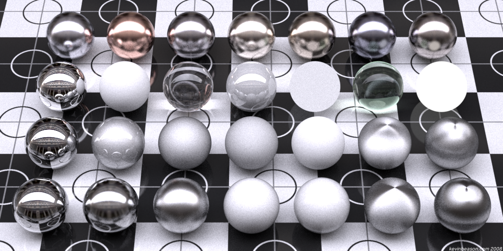
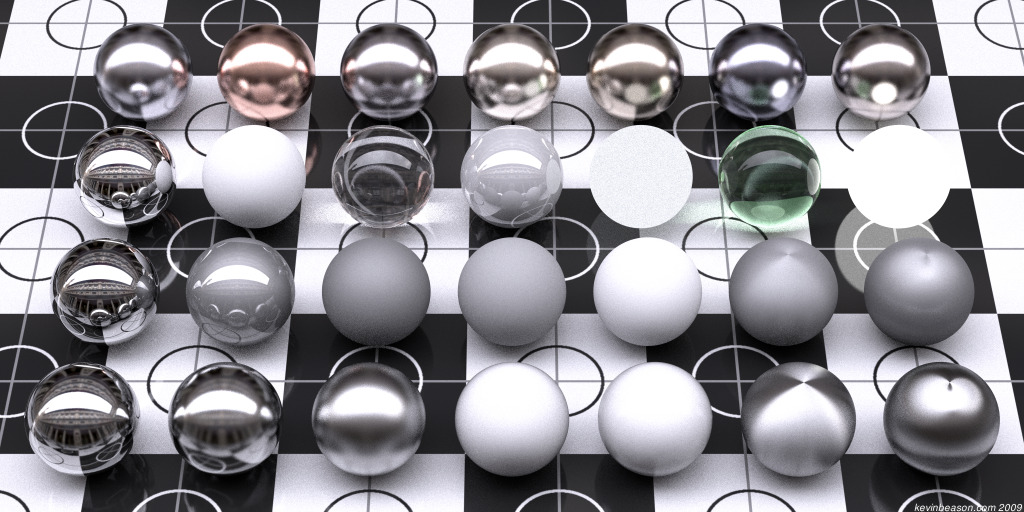
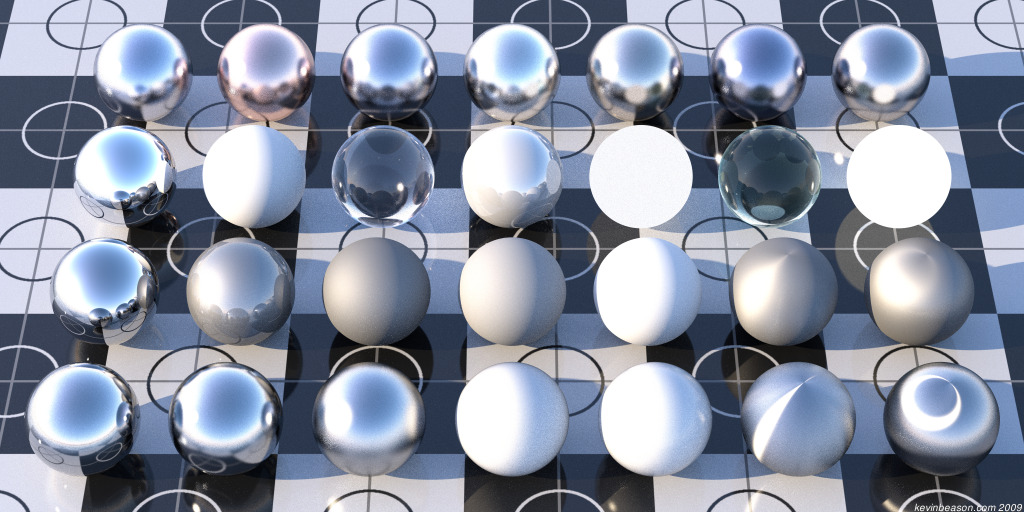
Added Ashikhmin & Shirley’s Anisotropic Phong BRDF and Schlick’s BRDF (the ’94 paper) support for pure path tracing (implicit light paths only). My Schlick BRDF is probably broken. Adding these entailed abstracting a BRDF interface class, implementing importance sampling and computing BRDF/PDF. The daylight image is after sunset for a good reason. The sun would only contribute if a ray found it by chance… talk about noise.
Front row is Ashikhmin & Shirley Anisotropic Phong BRDF. 2nd row is Schlick’s anisotropic BRDF. Third row is my preexisting set of materials. Back row is A&S BRDF with measured reflectance values (in RGB. See previous post.) The floor is A&S BRDF and my fascimile of their texture.
Left image is Preetham daylight model. Right is Debevec’s Uffizi HDR environment probe.
2048 spp, 24-30 minutes each on a Q6600 2.4GHz Core 2 Quad.
This work is from May 2008.
8 comments